Fundamentals of being an AI/ML sorcerer supreme

TLDR

Harnessing the power of AI can be magical and impactful. Before mastering this ability, one must understand the basic foundation of AI. We’ll go over basic math concepts, common prediction types, and popular algorithms.

Math

• Vectors
• Matrix
• Cost function

Classification and regression

• Accuracy
• Precision
• Recall
• Mean absolute error
• Root mean squared error

Algorithms

• Linear regression
• Logical regression
• K-Nearest Neighbors
• Decision trees
• Random forest
• Support vector machines
• Neural network

Math

Mathematical equations lay the foundation for AI. For basic applications of AI, being a math expert isn’t necessary as there are plenty of tutorials and pre-built libraries maintained by the open source community. However, learning some math concepts will help you understand why an algorithm works the way it does and how it can be improved.

Vectors

Vectors are an array of numbers (x = [1, 3, 5]), compared to a scalar which is a single number (x = 5).

A vector is a mathematical way of getting from one point to another. Vectors need to travel some distance which is measured in magnitude (length) and direction (orientation).

Vectors are used in machine learning for their ability to organize data. One example of a commonly used vector in machine learning is a feature vector. These contain information on multiple elements of an entity; for example, a feature vector can contain 5 values: the age of a user, the gender of a user, their height, their weight, and their current city. Feature vectors represent attributes of an entity in a way that a machine learning model can easily perform calculations on.

Vectors are written into Python using Numpy. They can be created using the function np.array():

Vectors can be added, subtracted, divided, multiplied, etc.

Matrix

A Matrix is a 2-dimensional array (table) of numbers with at least one column and at least one row. The array in a matrix can be represented as having m columns and nrows; therefore, our matrix is size m x n. A vector can also be considered a matrix. Row vectors can be represented as 1 x n, and column vectors as m x 1 .

A matrix is measured by its size which is the number of rows by the number of columns.

Matrices are used to represent data that machine learning models learn from. By structuring the data in a matrix, machine learning algorithms can leverage linear algebra and matrix multiplication for efficient calculations across large amounts of data.

In Python, a matrix is represented by a 2-D Numpy array:

Like vectors, matrices can be added, subtracted, divided, multiplied, etc. Matrices of the same size are added together by adding the corresponding data points.

Cost function

Cost function is used to optimize a machine learning model to make better predictions. The cost function calculates the error between predicted outcomes compared with actual outcomes. The goal of training a machine learning model is to minimize the error from this cost.

Gradient descent

To minimize the cost function error so a line best fits the dataset, we need to use a gradient descent algorithm. Gradient descent is an optimization algorithm that finds the minimum of a function — finding the value that’ll give us the lowest error.

Gradient descent works by taking steps to find the minimum value of the parabola graph.

As the graph slopes down towards the x-axis, theta (measure of an angle) will increase as the negative slope is turned positive by alpha. As the graph goes up past the minimum, theta will become negative, signaling it has passed the minimum and needs to backtrack. Repeatedly running this algorithm will leave us with the minimum.

Classification and Regression

There are 2 main categories that most machine learning problems belong to: classification and regression.

Classification is the process of taking an input and mapping it to a discrete label. Classification problems typically deal with classes or categories. For example, a photo of a cat (input) and mapping it to be labeled either cat or dog.

Regression allows us to predict a continuous outcome variable based on predictor variables. Generally, regression problems deal with real numbers. For example, trying to predict home prices based on recent sales in an area.

Evaluation metrics explain the performance of a model and can provide insight to areas that might need improvement.

In our example, we built an ML model to predict a color. Every time the model chooses a color, a score will be added to their box. Actual values are on the y-axis and the model’s predicted values are on the x-axis.

Classification evaluation metrics

Accuracy

Accuracy is the total number of correct predictions divided by the total number of predictions made by the model. Accuracy works well on balanced data: a dataset with approximately the same number values across each category present. For example, 100 dogs and 95 cats is a balanced dataset. An unbalanced dataset is 100 dogs and 11 cats.

18 (correct predictions) / 22 (total number of predictions) = 0.81
Accuracy = 81%

15 (correct predictions) / 22 (total number of predictions) = 0.68
Accuracy = 68%

Classification accuracy can give a false sense of achieving high performance. Such can occur when there is a disproportionate number of 1 color over the other (e.g. 100 blues and only 11 reds).

Models can be evaluated based on four features:

1. True positives are the correctly identified predictions for each class.
2. True negatives are the correctly rejected predictions for each class.
3. False positives are incorrectly identified predictions for each class.
4. False negatives are incorrectly rejected data for each class.

Precision

Precision is the number of correct positive results divided by the number of positive results predicted by the ML model. Using precision, we discover the amount of positive identifications that were actually correct. Precision is helpful for understanding how good a model is at predicting a specific category. This metric is helpful in multi-category classification problems. For example, predicting which color car to sell.

Precision = True positive / (True positives + False positive)

Referring back to our model 1 color identifier from above, the true positive value would be 10 and the false positive value would be 3.

Precision = 10 / (10 + 3) = 0.769
Precision = 77%

Recall

Recall is the number of all positive results divided by the number of all relevant samples. Recall answers the question: what proportion of actual positives were identified correctly? A model that produces no false negatives has a recall of 1. Recall is useful when assessing whether a model can effectively detect the occurrence of a specific category. For example, if you need a model that can catch all fraudsters on your website then you’ll want a model that has high recall. A model with high recall may have low precision (gets a lot of predictions wrong) but it’s really good at detecting all the fraudsters.

Recall = True positive / (True positive + False negative)

Referring to our color identifier model, the true positives are again 10 and the false negative is 1.

Recall = 10 / (10 + 1) = 0.909
Recall = 91%

F1 Score

F1 score tries to find the balance between precision and recall. It tells how precise and robust a classifier is and ranges on a scale of [0,1]. The greater the F1 score, the better the performance of the model.

Regression evaluation metrics

Regression measures the relation between values of one variable and the corresponding values of another. An example of a regression could be the number of hours spent studying (x-axis) to the score received on an exam (y-axis).

Mean absolute error

Mean absolute error measures how far predicted values are from observed values averaged over all predictions.

In our example, our model will be based on predicted grocery item prices vs the actual grocery item prices.

The error can be predicted as: actual cost — predicted cost. After subtracting the two, we change any negative number to a positive by taking the absolute value of that number.

Apple = 2 − 1 = 1
Pasta = 3 − 5 = -2, absolute error = | -2 | = 2
Almond milk = 5 − 4 = 1, absolute error = | 1 | = 1
Avocado = 1 − 2 = -1, absolute error = | -1 | = 1
Ice cream = 5 − 3 = 2, absolute error = | 2 | = 2

The number of training sets in our data is 5; therefore, we will assign the variable n to equal 5.

MAE = (absolute error A + absolute error B + absolute error C + absolute error D + absolute error E) / n

MAE = (1 + 2 + 1 + 1 + 2) / 5 = 1.4

We’re therefore able to identify that our model predictions were off my $1.40 on average .

Root mean squared error

Root mean squared error is the square of the difference between the original values and the predicted values. A result from squaring errors is that larger errors become more pronounced.

Going off to our example above the RMSE would be as followed:

Apple = (2 − 1)^2 = 1
Pasta = (3 − 5)^2 = 4
Almond Milk = (4 − 5)^2 = 1
Avocado = (1 − 2)^2 = 1
Ice cream = (3 − 5)^2 = 4
RMSE = (1 + 4 + 1 + 1 + 4) / 5
RMSE = 2.2

Algorithms

There are many great algorithms, some are better than others depending on your use case or data availability. Here’s a useful visual diagram of when to use which algorithm:

https://scikit-learn.org/stable/tutorial/machine_learning_map/index.html

Here’s a brief overview of some of the more popular algorithms used below:

Linear regression

Regression models target values based on independent variables. Linear regression is a type of regression analysis where there’s a linear relationship between the independent and dependent variables.

By finding the linear relationship between values, machines are better able to forecast upcoming variables.

A simple linear regression would be the time spent studying (x-axis) to the grade received on a test (y-axis). Presumably, the most time spent studying would result in a higher grade.

Logistic regression

Tests whether an independent variable has an effect on a binary dependent variable. In ML, logistic regression is used as a classifier to execute tasks.

Logistic regression is used for its ability to provide probabilities which can be used to classify new data.

For example, logistic regression can be used to determine whether or not an email is spam. Spam emails will be categorized based on key words and features that show up in those emails. When new emails come in, it can determine whether or not it’s spam based on those identified characteristics.

K-Nearest Neighbors

Uses data points surrounding a target data point in order to make predictions about the target. It assumes that similar things exist in close proximity to each other.

KNN can be used in problems that are built on identifying similarities.

KNN can be used to identify patterns in buying behavior and enable businesses to use that to increase sales. For example, a grocery store can use KNN to identify the types of people who buy wine on Friday. The grocery store can find similar customers using this model and then tailor their marketing to that demographic.

Decision trees

We use decision trees in our everyday life when making choices. For example when buying a new car we usually decide on a price point and look for things below that point. Then we may choose the type of seats we want. Based on what is available with the type of seat we want, we choose the color car we want. Decision trees are commonly used when working with non-linear datasets.

Random forest

Creates an algorithm based on how many decision trees (creating the ‘forest’) are available. The more trees, the more accurate the algorithm’s prediction will be.

Random forest can cross validate inputs, thus, making its output more accurate. This algorithm is used when handling large datasets.

Stock traders can use decision forests to predict a stock’s future behavior. They do this by taking decision trees of similar stocks which cross validate each other’s input which can make predicting the potential of a new, similar stock more accurate.

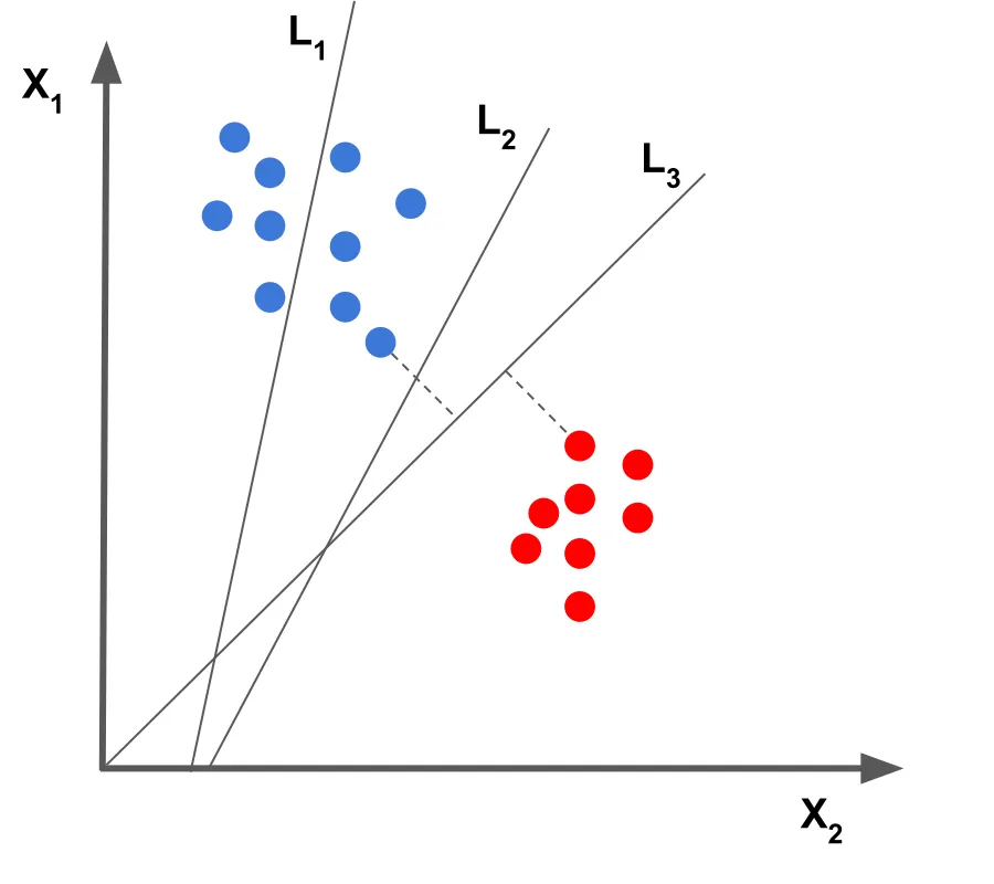
Support vector machines

Hyperplanes are decision boundaries used to classify data. Support vectors are data points lying closest to the decision line that are most difficult to classify. SVMs find an optimal solution to classify these data points.

SVMs have a high speed and high performance accuracy with a limited amount of data.

SVMs are being used to classify cancer using image classification. The SVM algorithm runs models with datasets of thousands of cancerous cell images. It classifies the image around the cell and after processing thousands of images, can accurately classify scans in real time.

Neural Network

Neural networks are a series of algorithms used to find relationships in data.Neural networks are able to learn by themselves, thus, have the ability to produce an output not limited to the given input. This algorithm has been implemented in image object detection, language understanding, audio detection, and more.

Neural networks have been used to teach a machine how to play chess. Analyzing over 2.5 million chess matches, this neural network predicts chess moves based on the history of moves in the game. This is significant because it demonstrates the ability of a machine to learn and understand game theory.

Conclusion

With the right foundation, developing AI/ML is an accessible goal. You’re now ready to start coding. Check out how to build your first machine learning model: https://m.mage.ai/how-to-get-started-with-ai-ml-8630fecfd776